现代卷积神经网络

import torch

from torch import nn

from d2l import torch as d2l

net = nn.Sequential(

    nn.Conv2d(1,96,kernel_size=11,stride=4,padding=1),nn.ReLU(),

    nn.MaxPool2d(kernel_size=3,stride=2),

    # 减小卷积窗口，使用填充 2 来使输入和输出一致且增大输出通道数

    nn.Conv2d(96,256,kernel_size=5,padding=2),nn.ReLU(),

    nn.MaxPool2d(kernel_size=3,stride=2),

    nn.Conv2d(256,384,kernel_size=3,padding=1),nn.ReLU(),

    nn.Conv2d(384,384,kernel_size=3,padding=1),nn.ReLU(),

    nn.Conv2d(384,256,kernel_size=3,padding=1),nn.ReLU(),

    nn.MaxPool2d(kernel_size=3,stride=2),

    nn.Flatten(),

    nn.Linear(6400,4096),nn.ReLU(),

    nn.Dropout(p=0.5),

    nn.Linear(4096,4096),nn.ReLU(),

    nn.Dropout(p=0.5),

    nn.Linear(4096,10)

)

X = torch.randn(1,1,224,224)

for layer in net:

    X = layer(X)

    print(layer.__class__.__name__,'output shape:\t',X.shape)

batch_size = 128

train_iter,test_iter = d2l.load_data_fashion_mnist(batch_size,resize=224)

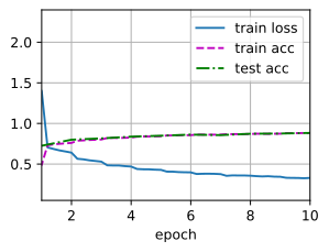
lr,num_epochs = 0.01,10

d2l.train_ch6(net,train_iter,test_iter,num_epochs,lr,d2l.try_gpu())

import torch

from torch import nn

from d2l import torch as d2l

def vgg_block(num_convs,in_channels,out_channels):

    layers = []

    for _ in range(num_convs):

        layers.append(nn.Conv2d(in_channels,out_channels,kernel_size=3,padding=1))

        layers.append(nn.ReLU())

        in_channels = out_channels

    layers.append(nn.MaxPool2d(kernel_size=2,stride=2))

    return nn.Sequential(*layers)

conv_arch = ((1,64),(1,128),(2,256),(2,512),(2,512))

def vgg(conv_arch):

    conv_blks = []

    in_channels = 1

    for (num_convs,out_channels) in conv_arch:

        conv_blks.append(vgg_block(num_convs,in_channels,out_channels))

        in_channels = out_channels

    return nn.Sequential(

        *conv_blks,nn.Flatten(),

        nn.Linear(out_channels * 7 * 7,4096),nn.ReLU(),nn.Dropout(0.5),

        nn.Linear(4096,4096),nn.ReLU(),nn.Dropout(0.5),

        nn.Linear(4096,10)

    )

net = vgg(conv_arch)

X = torch.randn(1,1,224,224)

for blk in net:

    X = blk(X)

    print(blk.__class__.__name__,'output shape:\t',X.shape)

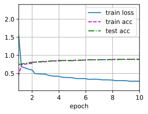
lr,num_epochs,batch_size = 0.01,10,128

train_iter,test_iter = d2l.load_data_fashion_mnist(batch_size,resize=224)

d2l.train_ch6(net,train_iter,test_iter,num_epochs,lr,d2l.try_gpu())

import torch

from torch import nn

from d2l import torch as d2l

def  nin_block(in_channels,out_channels,kernel_size,strides,padding):

    blk = nn.Sequential(

        nn.Conv2d(in_channels,out_channels,kernel_size,strides,padding),

        nn.ReLU(),

        # 后面两个是 1x1 的卷积层

        nn.Conv2d(out_channels,out_channels,kernel_size=1),

        nn.ReLU(),

        nn.Conv2d(out_channels,out_channels,kernel_size=1),

        nn.ReLU()

    )

    return blk

net = nn.Sequential(

    nin_block(1,96,kernel_size=11,strides=4,padding=0),

    nn.MaxPool2d(3,stride=2),

    nin_block(96,256,kernel_size=5,strides=1,padding=2),

    nn.MaxPool2d(3,stride=2),

    nin_block(256,384,3,1,1),

    nn.MaxPool2d(3,stride=2),

    nn.Dropout(0.5),

    nin_block(384,10,3,1,1),

    nn.AdaptiveAvgPool2d((1,1)),

    # 四维的输出转换成二维，(批量大小，10)

    nn.Flatten()

)

X = torch.rand(size=(1,1,224,224))

X

for layer in net:

    X = layer(X)

    print(layer.__class__.__name__,'output shape:\t',X.shape)

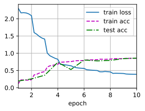
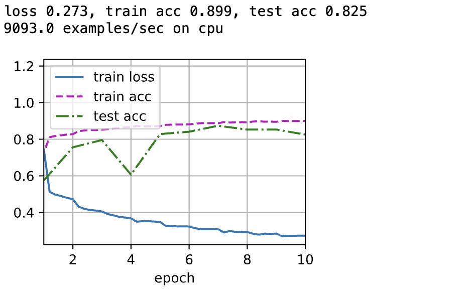
lr, num_epochs, batch_size = 0.1,10,128

train_iter,test_iter = d2l.load_data_fashion_mnist(batch_size,resize=224)

d2l.train_ch6(net,train_iter,test_iter,num_epochs,lr,device=d2l.try_gpu())

import torch

from torch import nn

from torch.nn import functional as F

from d2l import torch as d2l

class Inception(nn.Module):

    # c1--c4 是每条路径的输出通道数

    def __init__(self,in_channels,c1,c2,c3,c4,**kwargs):

        super(Inception,self).__init__(**kwargs)

        # 路径 1，单 1x1 卷积层

        self.p1_1 = nn.Conv2d(in_channels,c1,kernel_size=1)

        # 路径 2，1x1 卷积后接 3x3 卷积层

        self.p2_1 = nn.Conv2d(in_channels,c2[0],kernel_size=1)

        self.p2_2 = nn.Conv2d(c2[0],c2[1],kernel_size=1)

        # 路径 3，1x1 卷积层后链接 5x5 卷积层

        self.p3_1 = nn.Conv2d(in_channels,c3[0],kernel_size=1)

        self.p3_2 = nn.Conv2d(c3[0],c3[1],kernel_size=3,padding=1)

        # 路径 4，3x3 最大汇聚层后接入 1x1 卷积层

        self.p4_1 = nn.MaxPool2d(kernel_size=3,stride=1,padding=1)

        self.p4_2 = nn.Conv2d(in_channels,c4,kernel_size=1)

    def forward(self,x):

        p1 = F.relu(self.p1_1(x))

        p2 = F.relu(self.p2_2(F.relu(self.p2_1(x))))

        p3 = F.relu(self.p3_2(F.relu(self.p3_1(x))))

        p4 = F.relu(self.p4_2(self.p4_1(x)))

        return torch.cat((p1,p2,p3,p4),dim=1)

# GoogleNet 实现

# 第一个模块采用 64 通道，7x7 卷积层

b1 = nn.Sequential(

    nn.Conv2d(1,64,kernel_size=7,stride=2,padding=3),

    nn.ReLU(),

    nn.MaxPool2d(kernel_size=3,stride=2,padding=1)

)

# 第二个模块使用两个卷积层，第一个卷积层是 64 通道，1x1 卷积层，第二哥卷积层使用将通道数增加为 3 倍的 3❤3 卷积层

b2 = nn.Sequential(

    nn.Conv2d(64,64,kernel_size=1),

    nn.ReLU(),

    nn.Conv2d(64,192,kernel_size=3,padding=1),

    nn.ReLU(),

    nn.MaxPool2d(kernel_size=3,stride=2,padding=1)

)

'''

第三个模块串联两个完整的Inception模块

* 第一个Inception块的输出通道数为64+128+32+32=256，第二条和第三条路径首先将输入通道数分别减少到96/192=1/2,和16/192=1/12，然后链接第二个卷积层

* 第二个Inception块的输出通道数增加到128+192+96+64=480，第二条路径和第三条路径先将输入通道分别减少到128/256=1/2和32/256=1/8

'''

b3 = nn.Sequential(

    Inception(192,64,(96,128),(16,32),32),

    Inception(256,128,(128,192),(32,96),64),

    nn.MaxPool2d(kernel_size=3,stride=2,padding=1)

)

"""

第四个模块，串联5个Inception块，输出通道分别是192+208+48+64=512,160+224+64+64=512,128+256+64+64=512,112+288+64+64=528,256+320+128+128=832

"""

b4 = nn.Sequential(

    Inception(480,192,(96,208),(16,48),64),

    Inception(512,160,(112,224),(24,64),64),

    Inception(512,128,(128,256),(24,64),64),

    Inception(512,112,(144,288),(32,64),64),

    Inception(528,256,(160,320),(32,128),128),

    nn.MaxPool2d(kernel_size=2,stride=2,padding=1)

)

"""

第五个模块包含输出通道为256+320+128+128=832和384+384+128+128=1024的两个Inception块

后面紧跟输出层，使用全局平均汇聚层，将每个通道的高度和宽度变为1，再连接一个输出个数为标签类别数的全连接层

"""

b5 = nn.Sequential(

    Inception(832,256,(160,320),(32,128),128),

    Inception(832,384,(192,384),(48,128),128),

    nn.AdaptiveAvgPool2d((1,1)),

    nn.Flatten(),

)

net = nn.Sequential(

    b1,b2,b3,b4,b5,

    nn.Linear(1024,10)

)

# GoogleNet 模型比较复杂，可以降低输入的高度和宽度

X= torch.rand(size=(1,1,96,96))

for layer in net:

    X = layer(X)

    print(layer.__class__.__name__,'output shape:\t',X.shape)

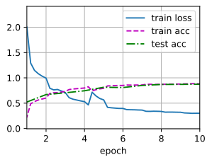
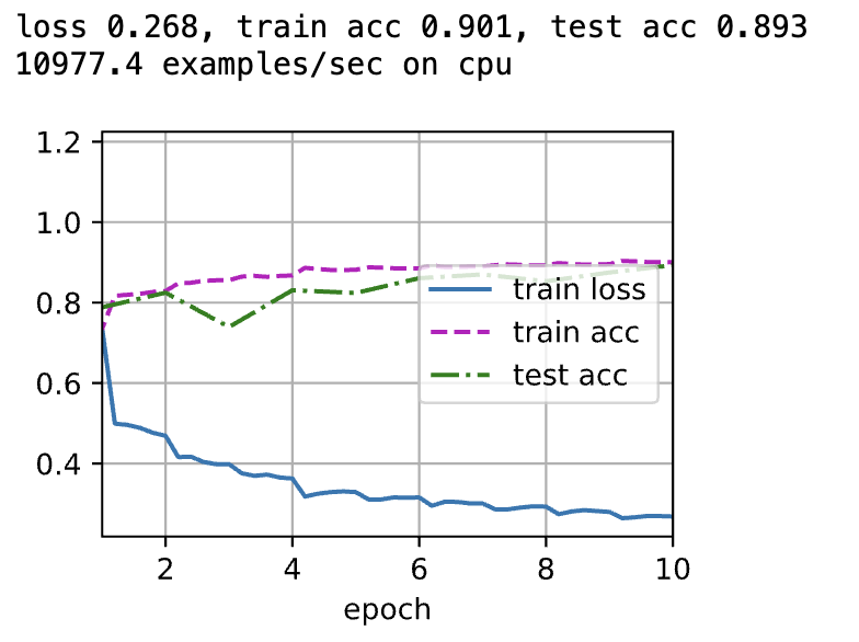
lr,num_epochs,batch_size = 0.1,10,128

train_iter,test_iter = d2l.load_data_fashion_mnist(batch_size,resize=96)

d2l.train_ch6(net,train_iter,test_iter,num_epochs,lr,d2l.try_gpu())

import torch

from torch import nn

from d2l import torch as d2l

def  batch_normal(X,gamma,beta,moving_mean,moving_var,eps,momentum):

    # 通过 is_grad_enabled 方法判断当前模式是训练模式还是预测模式

    if not torch.is_grad_enabled():

        # 如果是预测模式，直接使用传入的移动平均所得的均值和方差

        X_hat = (X-moving_mean)/torch.sqrt(moving_var+eps)

    else:

        assert len(X.shape) in (2,4)

        if len(X.shape) == 2:

            # 使用全连接层的情况，计算特征维上的均值和方差

            mean = X.mean(dim=0)

            var = ((X-mean)**2).mean(dim=0)

        else:

            # 使用二维卷积层的情况，计算通道维上 (axis==1) 的均值和方差

            # 保留 X 的形状以便后面做广播运算

            mean = X.mean(dim=(0,2,3),keepdim=True)

            var = ((X-mean)**2).mean(dim=(0,2,3),keepdim=True)

        # 训练模式下，使用当前的均值和方差做标准化

        X_hat = (X - mean) / torch.sqrt(var + eps)

        # 更新移动平均的均值和方差

        moving_mean = momentum * moving_mean + (1.0 - momentum) * mean

        moving_var = momentum * moving_var + (1.0 - momentum) * var

    Y = gamma * X_hat + beta # 缩放和移位

    return Y,moving_mean.data,moving_var.data

class BatchNorm(nn.Module):

    # num_features: 全连接层的输出数量或卷积层的输出通道数

    # num_dims: 2 表示完全连接层，4 表示卷积层

    def __init__(self,num_features, num_dims):

        super().__init__()

        if num_dims == 2:

            shape = (1, num_features)

        else:

            shape = (1, num_features, 1, 1)

        # 参与求梯度和迭代的拉伸参数和偏移参数，其分别初始化为 1 和 0

        self.gamma = nn.Parameter(torch.ones(shape))

        self.beta = nn.Parameter(torch.zeros(shape))

        # 非模型参数的变量初始化为 0 和 1

        self.moving_mean = torch.zeros(shape)

        self.moving_var = torch.ones(shape)

    def forward(self, X):

        # 如果 X 不在内存上，将 moving_mean 和 moving_var 复制到 X 所在的显存上

        if not self.moving_mean.device == X.device:

            self.moving_mean = self.moving_mean.to(X.device)

            self.moving_var = self.moving_var.to(X.device)

        # 保存更新过的 moving_mean 和 meaning_var

        Y,self.moving_mean,self.moving_var = batch_normal(

            X,self.gamma,self.beta,self.moving_mean,self.moving_var,eps=1e-5,momentum=0.9)

        return Y

net = nn.Sequential(

    nn.Conv2d(1,6,kernel_size=5),BatchNorm(6,4),nn.Sigmoid(),

    nn.AvgPool2d(kernel_size=2,stride=2),

    nn.Conv2d(6,16,kernel_size=5),BatchNorm(16,4),nn.Sigmoid(),

    nn.AvgPool2d(kernel_size=2,stride=2),nn.Flatten(),

    nn.Linear(16*4*4, 120),BatchNorm(120,2),nn.Sigmoid(),

    nn.Linear(120, 84),BatchNorm(84,2),nn.Sigmoid(),

    nn.Linear(84, 10)

)

lr,num_epochs,batch_size = 1.0,10,256

train_iter, test_iter = d2l.load_data_fashion_mnist(batch_size)

d2l.train_ch6(net,train_iter,test_iter,num_epochs,lr,d2l.try_gpu())

net[1].gamma.reshape((-1,)),net[1].beta.reshape((-1,))

net = nn.Sequential(

    nn.Conv2d(1,6,kernel_size=5),nn.BatchNorm2d(6),nn.Sigmoid(),

    nn.AvgPool2d(kernel_size=2,stride=2),

    nn.Conv2d(6,16,kernel_size=5),nn.BatchNorm2d(16),nn.Sigmoid(),

    nn.AvgPool2d(kernel_size=2,stride=2),nn.Flatten(),

    nn.Linear(16*4*4, 120),nn.BatchNorm1d(120),nn.Sigmoid(),

    nn.Linear(120, 84),nn.BatchNorm1d(84),nn.Sigmoid(),

    nn.Linear(84, 10)

)

d2l.train_ch6(net,train_iter,test_iter,num_epochs,lr,d2l.try_gpu())

import torch

from torch import nn

from torch.nn import functional as F

from d2l import torch as d2l

class Residual(nn.Module):

    def __init__(self, input_channels, num_channels, use_1x1conv=False, strides=1):

        super().__init__()

        self.conv1 = nn.Conv2d(input_channels, num_channels, kernel_size=3, stride=strides, padding=1)

        self.conv2 = nn.Conv2d(num_channels, num_channels, kernel_size=3, stride=1, padding=1)

        if use_1x1conv:

            self.conv3 = nn.Conv2d(input_channels, num_channels, kernel_size=1, stride=strides)

        else:

            self.conv3 = None

        self.bn1 = nn.BatchNorm2d(num_channels)

        self.bn2 = nn.BatchNorm2d(num_channels)

    def forward(self, x):

        Y = F.relu(self.bn1(self.conv1(x)))

        Y = self.bn2(self.conv2(Y))

        if self.conv3 is not None:

            x = self.conv3(x)

        # 放在最后一层激活之前

        Y = Y + x

        return F.relu(Y)

blk = Residual(3,3)

X = torch.rand(4,3,6,6)

Y = blk(X)

Y.shape

blk = Residual(3,6,use_1x1conv=True,strides=2)

blk(X).shape

b1 = nn.Sequential(nn.Conv2d(1,64,kernel_size=7, stride=2,padding=3),nn.BatchNorm2d(64),nn.ReLU(),nn.MaxPool2d(kernel_size=3, stride=2,padding=1))

def resnet_block(in_channels, out_channels, num_residuals,first_block=False):

    blk = []

    for i in range(num_residuals):

        if i == 0 and not first_block:

            blk.append(Residual(in_channels, out_channels, use_1x1conv=True,strides=2))

        else:

            blk.append(Residual(out_channels, out_channels))

    return blk

b2 = nn.Sequential(*resnet_block(64,64,2,first_block=True))

b3 = nn.Sequential(*resnet_block(64,128,2))

b4 = nn.Sequential(*resnet_block(128,256,2))

b5 = nn.Sequential(*resnet_block(256,512,2))

net = nn.Sequential(b1,b2,b3,b4,b5,nn.AdaptiveAvgPool2d((1,1)),nn.Flatten(),nn.Linear(512,10))

X = torch.rand(size=(1,1,224,224))

for layer in net:

    X = layer(X)

    print(layer.__class__.__name__,'output shape:\t',X.shape)

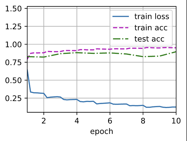
lr,num_epochs,batch_size = 0.05,10,256

train_iter, test_iter = d2l.load_data_fashion_mnist(batch_size)

d2l.train_ch6(net,train_iter,test_iter,num_epochs,lr,d2l.try_gpu())

import torch

from torch import nn

from d2l import torch as d2l

def conv_block(in_channels,num_channels):

    return nn.Sequential(nn.BatchNorm2d(in_channels),nn.ReLU(),

                         nn.Conv2d(in_channels,num_channels,kernel_size=3,stride=1,padding=1))

class DenseBlock(nn.Module):

    def __init__(self,num_convs,input_channels,num_channels):

        super(DenseBlock,self).__init__()

        layers = []

        for i in range(num_convs):

            layers.append(conv_block(num_channels * i + input_channels,num_channels))

        self.net = nn.Sequential(*layers)

    def forward(self,X):

        for blk in self.net:

            Y = blk(X)

            # 连接通道维度上每个卷积块的输入和输出

            X = torch.cat((X,Y),dim=1)

        return X

blk = DenseBlock(2,3,10)

X = torch.rand(4,3,8,8)

Y = blk(X)

Y.shape

def transition_block(in_channels,num_channels):

    return nn.Sequential(nn.BatchNorm2d(in_channels),nn.ReLU(),nn.Conv2d(in_channels,num_channels,kernel_size=1),nn.AvgPool2d(kernel_size=2,stride=2))

blk = transition_block(23,10)

blk(Y).shape

b1 = nn.Sequential(nn.Conv2d(1,64,kernel_size=7,stride=2,padding=3),nn.BatchNorm2d(64),nn.ReLU(),nn.MaxPool2d(kernel_size=3, stride=2,padding=1))

num_channels,growth_rate = 64,32

num_convs_in_dense_blocks = [4,4,4,4]

blks = []

for i,num_convs in enumerate(num_convs_in_dense_blocks):

    blks.append(DenseBlock(num_convs,num_channels,growth_rate))

    # 上一个稠密块的输出通道

    num_channels += num_convs * growth_rate

    # 在稠密块之间添加一个过渡层，使通道数减半

    if i!=len(num_convs_in_dense_blocks)-1:

        blks.append(transition_block(num_channels,num_channels // 2))

        num_channels //= 2

net = nn.Sequential(b1,*blks,nn.BatchNorm2d(num_channels),

                    nn.ReLU(),

                    nn.AdaptiveAvgPool2d((1,1)),

                    nn.Flatten(),

                    nn.Linear(num_channels,10))

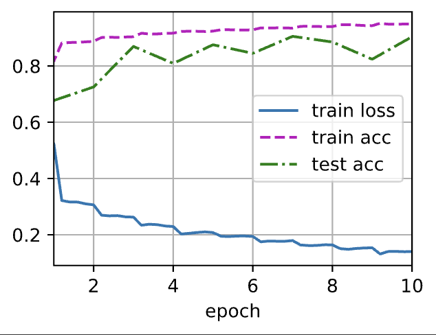
lr,num_epochs,batch_size = 0.1,10,256

train_iter, test_iter = d2l.load_data_fashion_mnist(batch_size,resize=96)

d2l.train_ch6(net,train_iter,test_iter,num_epochs,lr,d2l.try_gpu())